Simpler Machine Learning - Recurrent Neural Networks

Motivation for Recurrent Neural Networks

There exist applications where the inputs or outputs, or usually both, present themselves in a sequence of steps. Recurrent neural networks (RNNs) have been designed to deal with such applications. An example is the translation of text from one language to another. Suppose we want to translate the sentence “How do you do” into French. The input steps are the sequence of words: “How”, “do”, “you”, “do”. The output steps are the corresponding French words in sequence. Another example is translating the variations in air pressure in sequence over time that constitute spoken speech, into the corresponding written text. This application is called speech recognition, and it has recently become possible to get excellent speech recognition results using RNNs. It is possible to train an RNN to generate a novel corpus of text or body of music of a certain genre from scratch after having exposed it to a large body of sample text or music of that genre. We can take a sequence of raw DNA bases, and identify the protein sequences within that. We can take the sequence of words corresponding to the text of a movie review, and classify it as positive or negative, or give it a star rating from 1 to 5. This is called sentiment classification. There are a large number of such applications, and they are all enabled using RNNs.

Structure and Function of a Recurrent Neural Network

The diagram below shows the flow of information through an RNN.

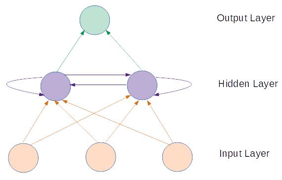
Each arrow, including the arrows feeding from the hidden layer neurons back into the hidden layer neurons, is a weight value. It is a number which is multiplied by the value feeding into it from the neuron before the weight to give a value feeding out of it into the neuron after the weight. The overall value flowing into a neuron is the sum of the values flowing into it from each of the arrows (weights). The neuron then performs a transformation on the value flowing into it to give the value flowing out of it. This diagram shows only two hidden layer neurons. In practice, there may be many more, and each hidden layer neuron is connected to every other hidden layer neuron.

We call the numerical value flowing out of a hidden layer neuron an “activation”. The value flowing into a hidden layer neuron is also an activation. The activation flowing into a hidden layer neuron is computed from the activations flowing out of all the hidden layer neurons including itself, and also from the weights feeding in from the input layer, using a certain method. This method lies at the heart of the working of an RNN. It is illustrated in the example below.

We start by introducing the idea of time steps. In a non-recurrent neural network, such as the XOR neural network presented earlier on this website, a single training example is presented to the neural network in a single pass through the network. The input values are presented to the input neurons in the input layer, and they feed forward to the output layer being multiplied by the weights and transformed by the neurons. The errors are then calculated and they propagate backwards through the network while updating the weights. That’s it for that training example. Likewise, while running the network on a sample not seen before, the input values are presented to the neurons in the input layer and they feed forward to the output layer to give the predicted values.

In a recurrent neural network, on the other hand, a single example is broken up into multiple time steps, and each of those time steps is presented in an individual pass through the network. Thus, it takes multiple steps to process a single example. For instance, consider a name entity recognition task. The goal is to identify the proper names in a sentence. Consider the sentence:

Among the presidents of America, Kennedy stands apart.

In our context, this is a single example. Each input of this one example will be one of the words above, in sequence, and each output will be the number 1 or 0 depending on whether the word is a proper name or not. To encode the input words as numerical vectors, we can create a dictionary (a vector is just a list of numbers; neural networks can only operate upon numbers). There are 8 words in the sentence above (we will ignore the punctuation). The first word, “Among”, is represented as [1,0,0,0,0,0,0,0]. The second word, “the”, is represented as [0,1,0,0,0,0,0,0]. The word “Kennedy” is represented as [0,0,0,0,0,1,0,0]. And so on. (In practice, the words will likely be encoded in alphabetical order). Such a representation is called a one-hot vector. In real life examples, with tens of thousands of words, the one-hot vectors will be in tens of thousands of dimensions instead of the 8 dimensions in our toy example.

Given all this, the input layer will now have 8 neurons. The output layer will have 1 neuron which will output a decimal number between 0 and 1. If the number is closer to 1, we will interpret that the input word is a proper name. If it is closer to 0, we will interpret that the input word is not a proper name. The hidden layer can have as many neurons as we deem reasonable, say 5 in our case.

We describe how we use this RNN to make predictions, assuming it is already trained. In the first time step of the input, we present the word “Among” ([1,0,0,0,0,0,0,0]) to the input layer. The hidden layer has 5 neurons, and thus 5 activations. The first time step of the input is the zeroth time step of the activations, and these are a vector of zeros ([0,0,0,0,0]). To get the output from the RNN for the first time step, we do a matrix multiplication to multiply the inputs by the input-to-hidden weights, the activations by the hidden-to-hidden weights, and feed the results into the hidden layer neurons. We then matrix multiply the values coming out of the hidden layer neurons by the hidden-to-output layer weights to get the value feeding into the output neuron. We transform the value feeding into the output layer neuron using something like a sigmoid function and get the final output of the neural network. Since the word “Among” is not a proper name, this should be a value closer to 0, say 0.12.

In the second time step, we present the word “the” ([0,1,0,0,0,0,0,0]) to the input layer, and pass it on to the hidden layer via the input-to-hidden weights. We also take the vector of activations from the first time step and feed it back into the hidden layer via the hidden-to-hidden weights. This time, the vector of activations will no longer be a zero vector; it will be a non-zero vector, like [0.71,0.43,-0.98,0.62,-0.37]. Again, since “the” is not a proper name, the output should be a number closer to 0.

When we come to the fifth time step, “America” ([0,0,0,0,1,0,0,0]), the vector of activations will come from the fourth time step. This time, the output should be a number closer to 1, say 0.93.

Now consider another example sentence from the above dictionary:

Kennedy stands.

This time we will input the word “Kennedy” in the first step ([0,0,0,0,0,1,0,0]) with a zero activation vector. We will input the word “stands” ([0,0,0,0,0,0,1,0]) in the second step using the activation vector from the first step. The RNN output for the first step should be close to 1, and the output for the second step should be close to 0.

Note that the number of words, or steps, in the second example is different from that in the first example. This is a fundamental and important property of RNNs. The number of time steps in different examples for the same neural network can be different. It is one of the major advantages of RNNs over vanilla neural networks.

We will not go over the training algorithm for RNNs in detail. If you review the training algorithm for the XOR neural network, you will see that the deltas are propagated backwards from the last layer to the first layer. Similarly, in an RNN, the deltas are propagated backwards from the last time step to the first time step. The training algorithm is called “backprogapagation through time”.

There are different varieties of RNNs. These are trained and run in slightly different ways. They are mentioned in the next section.

Types of Recurrent Neural Networks

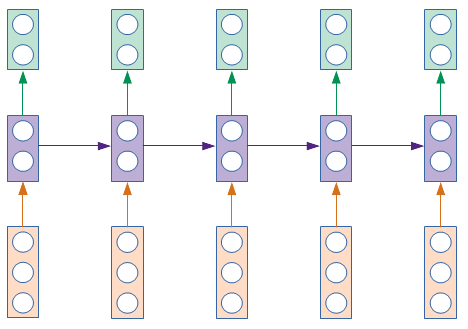
In the diagrams below, the vertical rectangles are vectors. The vector represents a layer of neurons. In the RNN structure shown in the above diagram, it took 12 arrows to show the weights between 6 neurons. For the diagrams that we will draw below, the information is dense enough that it is impractical to show the weight from every neuron to every other neuron. We will have to satisfy ourselves with showing a single arrow from one rectangle to the other. That arrow represents the entire set of weights from every neuron in the starting rectangle to every neuron in the ending rectangle. It is effectively a matrix, or a rectangular array of numbers. The mathematical operation being shown is a multiplication of the starting vector by the matrix to give the ending vector.

There are rectangles going from left to right. Each of the rectangles from left to right are the same layer. Each of the arrows from left to right are the same set of weights. The neural network is unrolled in time and spread out in space. This is done to make it easy to show the values flowing from the hidden layer back to itself across time steps. The orange rectangles are the input layer, the purple rectangles are the hidden layer, and the green rectangles are the output layer. They contain only a handful of neurons in the diagrams. In practice, there may be thousands of neurons.

The different types of RNNs are described below.

1. One to one

This is a vanilla neural network, like the XOR network. There is one time step of input, and one time time step of output.

2. One to many

A single input step generates multiple time steps of output. Generally, the output from each time step is fed back into the input of the next time step. Uses include generating a corpus of text or a body of music, of a certain genre.

3. Many to one

The inputs are fed in across multiple time steps, and result in a single time step of output. An example is sentiment classification. Each word of a text description is fed in one word at a time, and at the end, the RNN outputs a value giving a rating to the sentiment.

4. Many to many (synchronized)

The inputs and outputs are both spread across multiple time steps. For each input time step, there is a corresponding output time step. The name entity recognition application presented earlier in detail is an example use case.

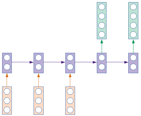
5. Many to many (not synchronized)

Again, the inputs and outputs are both spread across multiple time steps. But each input does not have a corresponding output. It may be the case that a sequence of inputs is presented first, and then a sequence of outputs is read out from the output. An example application is machine translation,where a sentence in one language is first read in, and a sentence in the translated language is then read out.

So that’s it for recurrent neural networks. There are many more details and subtleties that we have not covered. But hopefully this article gives you a basic idea about what an RNN is and how it works.